This is a condensed summary of “A Tutorial on (Co)Algebras and (Co)Induction” by Jacobs and Rutten. Note that this is for personal recall and hence unstructured.

Induction

A list with element type \(A\) is defined in Coq as the following:

Inductive list (A : Type) : Type :=
  | nil
  | cons (a : A) (l : list A).

The intuition for inductive definitions is that you start from a finite number of “constructors” and repeatedly apply them creating the elements of your definition. Thus the closure wrt the constructors becomes the definition.

The notion of constructors can be represented as an algebra which bunches together functions into a coproduct.

The constructors for \(\mathsf{list} \ A\) can be given the following signatures:

• \(\mathsf{nil} : 1 \rightarrow \mathsf{list} \ A\), where \(1\) denotes the unit type(no argument)
• \[\mathsf{cons} : A \times \mathsf{list} \ A \rightarrow \mathsf{list} \ A\]

The function cotuple \([\mathsf{nil}, \mathsf{cons}]\) is a interpretation(=implementation) of the T-functor(signature) \(T(X) = 1 + A \times X\) instantiated for athe carrier type \(\mathsf{list} \ A\). Together they for an algebra \(T(\mathsf{list} \ A) \rightarrow \mathsf{list} \ A : (\mathsf{list} \ A, [\mathsf{nil}, \mathsf{cons}])\) This means from the interpretation \(T(\mathsf{list} \ A)\) we can derive \(\mathsf{list} \ A\), or \(T(\mathsf{list} \ A) \rightarrow \mathsf{list} \ A\).

The functor \(T(X)\) above is a cotuple of two function signatures: \(1 \rightarrow X\) and \(A \times X \rightarrow X\). There are many algebras definable for the given functor, but we are interested in the one that gives us the “smallest” possible defintion of \(X\). Such “smallest” algebra gives us the smallest set of elements closed under its constructors, which naturally becomes the least fixed point of the functor(We’re just applying the constructors to create its elements). This is why an inductive definition is often described as the least fixpoint \(T(\mu x) \rightarrow \mu x\).

If we have a functor \(T(X) = X * X\), there’s no way to actually create an algebra from the given signature since we can’t start from anything that’s not in \(X\). Hence in this case the lfp and the initial algebra will be the empty type.

If we wish to do induction for a prop \(P \subseteq \mathsf{list} \ A\) over lists, we show the following:

• show \(P(\mathsf{nil})\) holds
• show \(P(l) \rightarrow P(a :: l)\) holds.

Suppose we set \(S_P := \{ l \ | \ P \ l\}\). The above proof is showing that \(\mathsf{nil} \in S_P\), and for any \(l \in S_P\), the results of applying the constructor should also be in \(S_P\). You can naturally see how the curry-howard correspondence appears here, in that a proof of \(P\) is equal to showing the construction of \(P \ x\) is possible (or is a member of \(S_P\) in views of sents).

If an algebra has an unique homomorphism to all other algebras of the given functor, it’s called the initial algebra of the functor. All the inductive types we define in coq are the initial algebra of their respective functors.

Initial algebras generalize the notion of the above sentence: “the results of applying the constructor should also be in \(S_P\)”.

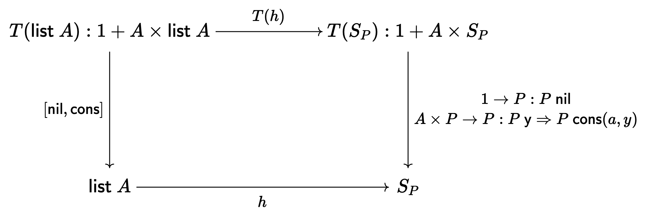
In the above picture we fixed \((\mathsf{list} \ A, [\mathsf{nil}, \mathsf{cons}])\) as the initial algebra. Initiality gives us the existence and uniqueness of homomorphism \(h\), and to prove \(P\) it suffices us to specialze the functor to \(S_P\), \(T(S_P)\), and defined \(T(S_P) \rightarrow S_P\). Because of the structure of \(T\), the structure \(T(S_P) \rightarrow S_P\) will be the same as the initial algebra, and hence be defined wrt its constructors.

In a nutshell algebras tell us that to define a function/prop for an inductive type defined by \(T(X)\), it suffices to define it along the structure of \(T(X)\). This sounds obvious but is showing that the underlying structure of an inductive type is universal.

Coinduction

Induction was a “construction”, going from a functor \(T(X)\) to its elements \(X\).

Coinduction is the exact opposite: \(X \rightarrow T(X)\). Given an element of type \(X\) that’s “already” a coinductive type, it gives us a set of functions \(T(X)\) which allows us to interact with it.

We can think of the underlying coinductive type element \(u\) to be some underlying, latent state we can’t directly access. But we’re allowed to apply some functions to it, so we can do things like get some observable value from the current state or advance the current state to another hidden state.

Consider the following functor:

The coalgebra with interpretation \(U \rightarrow T(U)\) and carrier \(U\) from the above functor gives us the following ways to interact with elements of \(U\):

• \(obs : U \rightarrow A\) : gives an observable output \(a \in A\) from the current state
• \(next : U \rightarrow U\) : move to the next underlying hidden state.

This is the exact opposite of induction, since induction gave us a way to construct elements of \(U\). But in coinduction we’re given a set of functions which pull out from the element. Induction describes the way how elements are constructed, while coinduction describes the way how elements can be destructed/interacted with.

Coinduction is sort of an extensinal view, in the sense that we’re not reasoning about the underlying object directly but just through its destructors/observable cases.

Just as homomorphisms between algebras existed and we had an initial algebra which had for all other algebras a unique homomorphism that connected the initial algebra to others, the dual of both concepts exist in coalgebras.

A final coalgebra is an algebra such for for all other coalgebras there exists a unique homomorphism from them to the final coalgebra. The homomorphism goes into the final coalgebra - opposite of iitial algebras:

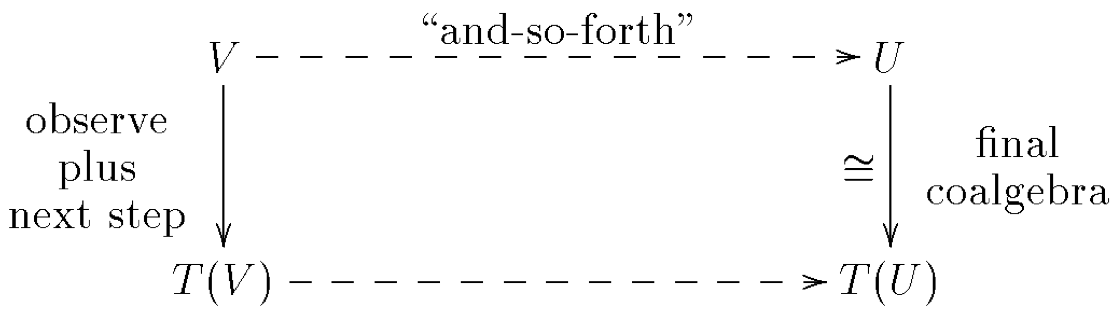
Now the final coalgebra is the greatest fixpoint \(\nu x \rightarrow T(\nu x)\) derivable from the functor and represents the “biggest” set of elements derivable. The intuition for why we need the gfp is because in an coinductive definition there’s always something to deconstruct, even after possibly applying a destructor infinite amount of times. So we need the “largest” constructions possible.

The tutorial mentions that functions/props defined on coinductive structures need to be defined wrt \(T(U)\) instead of \(U\) itself. This means in the case of streams, merging two streams \(u, u' \in U\) element-by-element becomes:

Note that we never reason about \(u, u'\) alone, but always enclosed in a destructor. This is the “blackbox” treatment of coinductive objects, and how it’s an extensional viewpoint.

Bisimulation takes this extensional viewpoint and creates a relation on two coinductive objects, saying that they are equal if they are “observationally equivalent” infinitely:

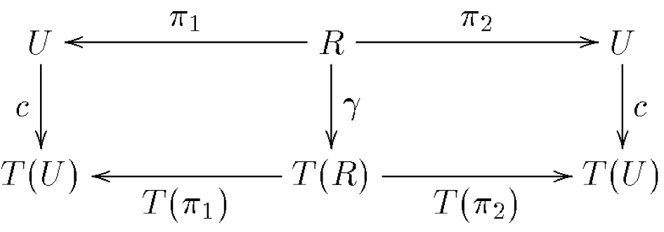
Here \(R \subseteq U \times U\) is a bisimulation relation on \(U\). Just like how for inductive types it required our prop to be defined on the structure \(T(X)\), we require our bisimulation relation to be defined on the functor \(T(U)\), fixing a coalgebra \(\gamma : R \rightarrow T(R)\).

In order for \(R\) to be a bisimulation, we need to show commutativity holds - projecting from \(R\)(\(\pi_1, \pi_2\)) and observing through \(c\) must be equal to first taking a step in the bisimulation through \(\gamma\) and then observing through \(T(\pi)\).

If \(c\) is a final coalgebra then \(R -> U\) must be unique, meaning \(\pi_1 = \pi_2\) under the carrier of the coalgebra. That is, if \(R(x, y)\) holds under a final coalgebra, \(x\) and \(y\) are identical under \(T(U)\).

Note that we just have to be able to construct a valid \(\gamma\) against a final coalgebra, and that’s the only necessary condition for showing equality under the final coalgebra.

생성(induction)과 관계(coinduction)의 건설 가능 여부(존재 여부) 자체가 증명.